Analysis and Visualization of Hyperpolarized 13C MR Data#
James Bankson1, Peder Larson2
1Department of Imaging Physics, The University of Texas MD Anderson Cancer Center; 2Department of Radiology and Biomedical Imaging, University of California, San Francisco
Abstract: Hyperpolarized 13C MR studies can provide powerful insight into the biochemistry of metabolism in vivo. Unlike traditional MRI contrast agents, the observable signal from HP agents is fleeting; magnetization is established in the polarizer, and once administered to the subject in the MRI scanner via bolus injection, magnetization is distributed through the body, depleted by signal excitations and lost to unavoidable spin-lattice relaxation. Acquisition strategies must be carefully planned to encode spatial, spectral, and temporal information within these constraints. Quantitative and semi-quantitative methods that are used to characterize signal evolution seek to distill complex multi-dimensional data into imaging biomarkers that reflect the unique information that is revealed by these agents, broadly reflecting the rate at which the precursor HP agent is metabolized to specific chemical endpoints. Intrinsic registration with traditional anatomic and functional 1H MRI provides critical context for the resulting metabolic imaging biomarkers. This chapter covers common approaches for HP data analysis, including common metrics and kinetic models, and guidance on how to visualize and navigate through HP data.
Key Words: Quantification, Pharmacokinetic Modeling, Kinetic Modeling, Ratiometric analysis, High-dimensional visualization
Data Extraction#
The key, and somewhat obvious, first step is to extract relevant data for analysis. In the case of HP 13C, we want to start our analysis based on metabolite signal amplitudes, which are often dynamic as well as spatially localized. In some cases this is trivial – when using imaging-based acquisition strategies, such as echo-planar or spiral imaging (see Hyperpolarized Acquistion Methods), this information is provided directly from the images themselves. When using spectroscopic-based acquisition techniques, such as MRS or MRSI, the metabolite amplitudes must be extracted from the spectral dimension. This is a common task in NMR/MR spectroscopy, thus it is recommended to use tools from this field. The ‘LCModel’ package (1) is an excellent choice, but requires choice of a basis set. For sparse spectra found in many HP studies (e.g. [1-13C]pyruvate), metabolite amplitudes can also be simply extracted integrating the area under the spectral peaks, or by fitting those peaks to Lorentzian lineshapes.
Another common task for analysis is to combine voxel data for region of interest (ROI) based computations, which requires knowledge of the anatomical location (see Data Visualization). It is important to note in the data extraction whether magnitude-only or complex-valued data is used, as they have different noise statistics that should be considered. Imaging sequences are typically stored as magnitude data, which has a Rician noise distribution (2, 3) with non-zero mean noise in regions of low signal. For low SNR data, mischaracterization of non-zero noise as signal can lead to biased results. This problem can be avoided by retrieving complex data when possible (4), or accounted for with maximum likelihood estimators (5) or power analysis methods (6).
Noise characteristics are also altered when combining data from multiple RF coils, and with undersampled or non-linear image reconstructions such as parallel imaging or compressed sensing. However, it is typically sufficient to assuming a Gaussian or Rician distribution, as these distributions become quite difficult to characterize.
Data Visualization#
Typically the next step following data extraction is data visualization for the purposes of anatomical localization, quality control, and/or qualitative evaluation. Good visualization requires co-registration with anatomical reference images from 1H MRI and also support for viewing additional dimensions including spectral (for spectroscopy-based acquisitions), metabolite (for imaging-based acquisitions), and temporal (for time-resolved acquisitions) dimensions. This enables matching HP data with underlying structures for analysis. Rapid visualization of data also allows for quality control after an experiment (“Did it work? Is there signal and is it approximately where we expect?”), and is important for presenting results especially within radiology and the imaging community.
For spectroscopy-based acquisitions, inherent visualization tools on human MRI scanners currently provide fairly limited functionality, and even tools on preclinical systems are often not sufficient for HP studies, especially when acquiring uniquely HP data such as time-resolved MRSI. Many investigators develop their own software infrastructure for visualization and analysis using their favorite scientific computing environment, but several packages are available for this purpose. One tool that includes specific features for HP 13C data is the SIVIC open-source software package (7, 8) (Figure 1). SIVIC reads MRI and MRSI DICOM images as well as multiple vendor specific raw data formats. The package runs on Windows, Linux and Mac and can be used for offline analyses. It can also run on a variety of scanner consoles (GE, Bruker, Agilent), and also can be used as a plug-in with OsiriX (9) and Horos (10). There are also several other popular packages for 1H MRSI that can be applied to HP 13C and includes jMRUI (11) and TARQUIN (12, 13).
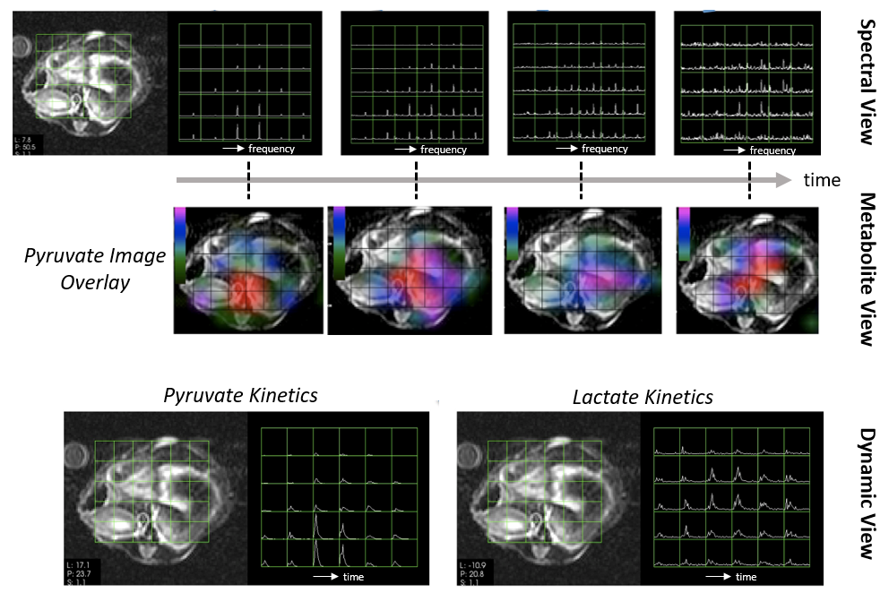
Figure 1: HP 13C Visualization modes. In this example, dynamic HP 13C MRSI data acquired covering mouse kidneys following HP [1-13C]pyruvate injection is displayed in three different modes, all of which are useful for visualization. These include displaying a time series of spectroscopic images (top), time series of metabolite maps extracted from the spectra (middle, shown as color overlay on T2-weighted anatomical images) and dynamic views showing the evolution of the HP signal from individual resonances through time (bottom). Visualizations were created with SIVIC. Figure adapted from Crane JC, et al. NMR in Biomedicine 2020, (14).
For imaging-based acquisitions, there are many common imaging tools that can support overlaying different images as this is a common task for PET/CT or multi-parametric MRI data. Some good tools include OsiriX and its free, open-source cousin, Horos, and ImageJ originally developed at the NIH, just to name a few.
Kinetic Modeling#
Signal from HP imaging agents behaves quite differently compared to traditional MRI. Magnetization is established in the polarizer at a level that can be four or five orders of magnitude greater than expected at thermal equilibrium, and once the HP agent is exposed to cells or reactants, or injected into a biological system, magnetization evolves continuously and dynamically over the visible lifetime of the agent. HP magnetization is not renewable in vivo; it is depleted by signal excitation pulses that convert stored longitudinal magnetization into observable transverse magnetization, and lost via spin-lattice (\(T_1\)) relaxation that continually acts to reduce magnetization towards thermal equilibrium.
Pharmacokinetic (PK) models can be used to describe the fate of imaging agents in biological systems. PK models for HP imaging agents are particularly important because they provide a framework to understand, explain, and quantify signal evolution in vivo. PK models for HP imaging agents should account for all sources of signal, and all loss mechanisms, and transition between spatial and chemical pools as accurately as possible. However, it should also be recognized that even the best and most complete PK model is an approximation, and that it is possible to generate models that are excessively complex and that may contain more unknowable parameters than our observed data can support. Over the next several sections, we’ll derive a set of PK models for HP pyruvate, which is the most widely used of all HP imaging agents to date and as of the writing of this chapter, the only HP agent that has been administered to human subjects. The process that we outline for establishing these PK models can easily be adapted for other HP imaging agents and metabolic pathways.
Modeling the chemical reaction#
Hyperpolarized [1-13C]-pyruvate is the most widely used HP imaging agent because it has good polarization characteristics (25-50% using current dDNP technology), a relatively long spin-lattice relaxation time constant (\(T_1\) ~ 60s at 3T), and because pyruvate is rapidly absorbed into tissue and incorporated into important metabolic pathways (Also see HP Agents and Biochemical Interactions). The conversion of HP [1-13C]-pyruvate into HP [1-13C]-lactate is particularly interesting in oncology because many cancers are characterized by high levels of aerobic glycolysis, or the Warburg Effect, where glucose is metabolized to lactate even under normoxic conditions (Also see Integration into Cancer Studies). Metabolism of HP pyruvate has been shown to provide unprecedented insight into the biochemistry of tumor metabolism in vivo, informing on tumor stage, aggressiveness, and response to therapy in a wide range of preclinical studies as discussed in the later chapters in this book.
Pyruvate and lactate are endogenous metabolic compounds that exist in dynamic equilibrium in all cells. Chemical conversion between pyruvate and lactate is mediated in cytosol by lactate dehydrogenase (LDH) and nicotinamide adenine dinucleotide (NADH) via an ordered ternary complex that has been well characterized (15). At equilibrium, there is no net conversion of pyruvate and lactate, but the two chemical pools are in continuous exchange; pyruvate molecules are converted into lactate at the same rate that lactate molecules are converted back into pyruvate. The equilibrium velocity of this reaction, \(V_{\text{LDH}}\) (mol/s), is a function of the concentrations of pyruvate, lactate, LDH, and NADH, and the kinetics of their interactions. When a pool of pyruvate molecules carrying a spin label enters into the system, as may be accomplished by administration of a quantity of HP pyruvate, then exchange of that spin label between chemical pools depends on the velocity of the underlying reaction, and on the likelihood of labeled molecules to participate in the reaction. If labeled molecules are uniformly mixed among endogenous molecules, then the probability of a labeled molecule entering into this reaction is simply the ratio of labeled molecules to the total number of molecules in that chemical pool. With that information, we can write a differential equation to describe the rate of change of labeled molecules (here, indicated with an asterisk) in each chemical pool:
\(\frac{\partial\text{Pyr}_{\text{ic}}^{*}(t)}{\partial t} = V_{\text{LDH}}\frac{\text{Lac}_{\text{ic}}^{*}(t)}{\text{Lac}_{\text{ic}}(t) + \text{Lac}_{\text{ic}}^{*}(t)} - V_{\text{LDH}}\frac{\text{Pyr}_{\text{ic}}^{*}(t)}{\text{Pyr}_{\text{ic}}(t) + \text{Pyr}_{\text{ic}}^{*}(t)}\) (1)
\(\frac{\partial\text{Lac}_{\text{ic}}^{*}(t)}{\partial t} = V_{\text{LDH}}\frac{\text{Pyr}_{\text{ic}}^{*}(t)}{\text{Pyr}_{\text{ic}}(t) + \text{Pyr}_{\text{ic}}^{*}(t)} - V_{\text{LDH}}\frac{\text{Lac}_{\text{ic}}^{*}(t)}{\text{Lac}_{\text{ic}}(t) + \text{Lac}_{\text{ic}}^{*}(t)}\) (2)
The subscripts on pyruvate and lactate in the equations above indicate that this reaction takes place only inside of cells.
Unfortunately, in a typical MR measurement following administration of HP pyruvate, we don’t have enough information about the endogeneous pool sizes for pyruvate and lactate, or the concentration of the coenzymes that mediate the reaction. Instead, exchange between these two pools is generally described using a first-order reaction involving apparent rate constants for chemical conversion. These reaction rate constants can be written as a function of the velocity of the reaction and the total amount of labeled and unlabeled molecules within each pool (16):
\(k_{\text{PL}} \equiv \frac{V_{\text{LDH}}}{\text{Pyr}_{\text{ic}}(t) + \text{Pyr}_{\text{ic}}^{*}(t)}\) (3)
\(k_{\text{LP}} \equiv \frac{V_{\text{LDH}}}{\text{Lac}_{\text{ic}}(t) + \text{Lac}_{\text{ic}}^{*}(t)}\) (4)
Substitution leads to the familiar first-order differential equation for two-site exchange.
\(\frac{\partial\text{Pyr}_{\text{ic}}^{*}(t)}{\partial t} = k_{\text{LP}}\text{Lac}_{\text{ic}}^{*}(t) - k_{\text{PL}}\text{Pyr}_{\text{ic}}^{*}(t)\) (5)
\(\frac{\partial\text{Lac}_{\text{ic}}^{*}(t)}{\partial t} = k_{\text{PL}}\text{Pyr}_{\text{ic}}^{*}(t) - k_{\text{LP}}\text{Lac}_{\text{ic}}^{*}(t)\) (6)
Modeling the biophysical system#
HP imaging agents such as pyruvate are administered into biological systems via intravenous injection, and must overcome multiple barriers before they arrive and interact with biological targets that we seek to interrogate. For example, membrane transport in and out of cells (15, 17, 34) as well as pyruvate delivery (18, 19)have been shown to play an important role in many HP experimental settings. Our pharmacokinetic models must also account for the effects of these barriers.
Fick’s law governs the flux of an imaging agent along a concentration gradient. One of the consequences of this law is that the flux of an imaging agent across a membrane can be written as a function of the difference in concentrations and the permeability of that membrane. For example,
\(j = P\left( \text{Pyr}_{\text{ee}}(t) - \text{Pyr}_{\text{ic}}(t) \right)\) (7)
relates the flux, j, or amount of pyruvate crossing between intracellular and extravascular/extracellular space (EES) per unit time, to the product of the concentration difference and P, the permeability of the cell membrane to pyruvate. Note that we have dropped the asterisk which signifies the pool of pyruvate that carries a spin label. From here forward, we recognize that only labeled pyruvate is visible in HP MR measurements.
The rate at which pyruvate enters cells is a product of this flux and the cross-sectional area between the two volume compartments, \(A\), and the change in concentration is found by dividing by the total volume of that compartment, \(V_{\text{ic}}\):
\(\frac{\partial\text{Pyr}_{\text{ic}}(t)}{\partial t} = j\frac{A}{V_{\text{ic}}} = \frac{\text{PA}}{V_{\text{ic}}}\left( \text{Pyr}_{\text{ee}}(t) - \text{Pyr}_{\text{ic}}(t) \right)\) (8)
We can simplify this expression by recognizing that the total intracellular volume can be written as a product of the total volume, \(V_{T}\), which may represent a voxel in an imaging measurement, and an intracellular volume fraction \((V_{\text{ic}} = v_{\text{ic}}V_{T};\ V_{\text{ee}} = v_{\text{ee}}V_{T})\) and defining a transfer rate constant that encapsulates the permeability of the boundary to the agent and the cross-sectional area between physical compartments, \(A_{\text{ec}}\), per unit volume. Defining an apparent rate constant \(k_{\text{ecp}} \equiv \frac{PA_{\text{ec}}}{V_{T}}\), we can write the coupled equations that describe the rate of change of HP pyruvate in both compartments, as illustrated in Figure 2.
\(\frac{\partial\text{Pyr}_{\text{ic}}(t)}{\partial t} = \frac{k_{\text{ecp}}}{v_{\text{ic}}}\left( \text{Pyr}_{\text{ee}}(t) - \text{Pyr}_{\text{ic}}(t) \right)\) (9)
\(\frac{\partial\text{Pyr}_{\text{ee}}(t)}{\partial t} = \frac{k_{\text{ecp}}}{v_{\text{ee}}}\left( \text{Pyr}_{\text{ic}}(t) - \text{Pyr}_{\text{ee}}(t) \right)\) (10)
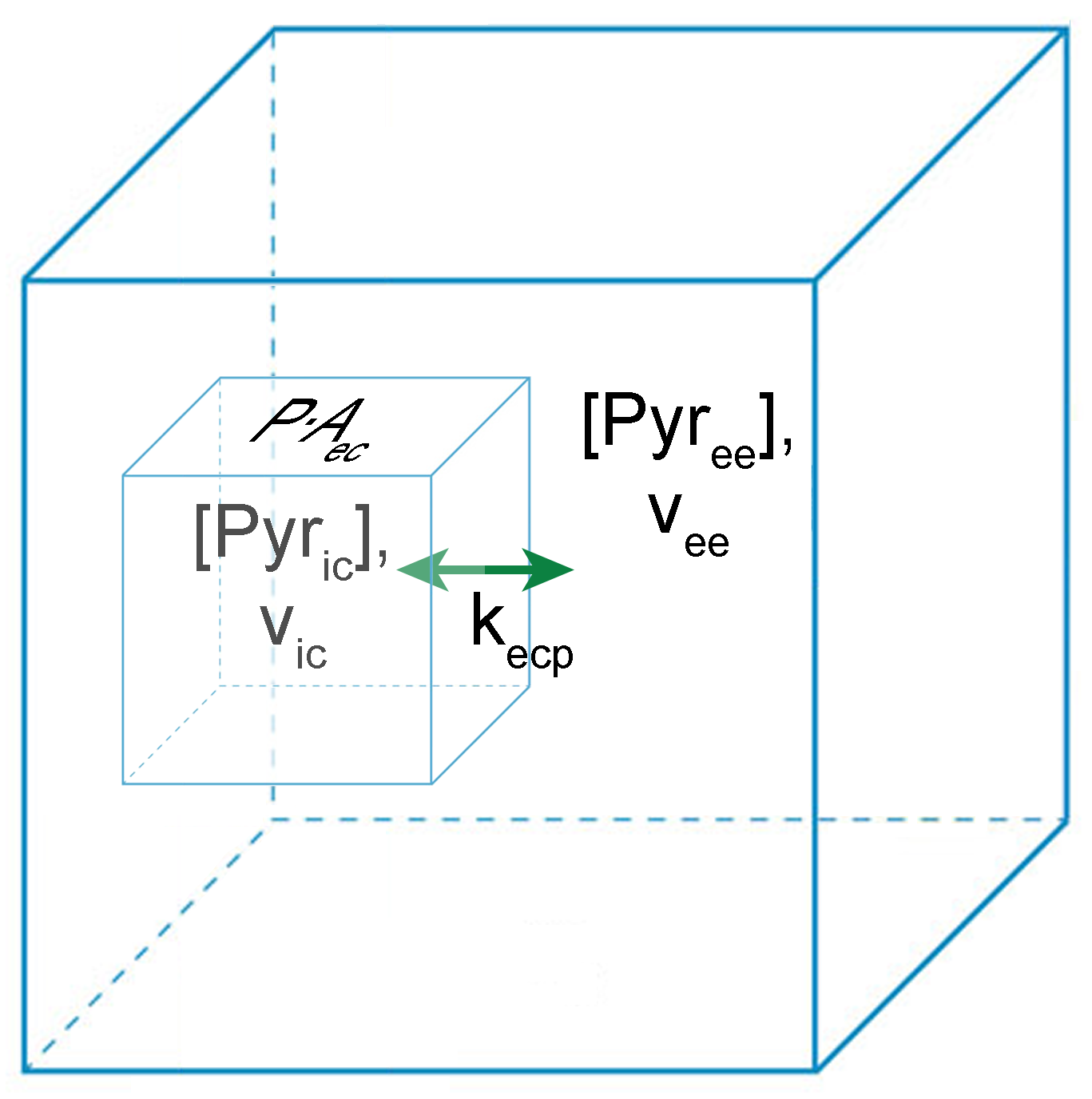
Figure 2: Transfer between physical compartments in a pharmacokinetic model. The rate of change in the concentration of pyruvate in intracellular space and extravascular/extracellular space is coupled, and depends on the difference in concentration in the two compartments, the relative volume of the two compartments, the permeability of the barrier between compartments to the agent, and the cross sectional area separating the two compartments. The outer blue cube represents the total volume, while the inner blue cube represents the intracellular volume and the barrier between the two subvolumes.
The PK model that we ultimately want to characterize is illustrated in Figure 3. In order to describe the movement of labeled spins between all physical compartments (intravascular, extravascular/extracellular, and intracellular) and chemical compartments (pyruvate and lactate), we need a description of the exchange between blood vessels and the EES. This can be written similarly to equations 10 and 11 but with the intravascular volume fraction, \(v_{b}\) and a rate contant, \(k_{\text{vee}}\), that represents the rate at which our HP imaging agents extravasate from vasculature to EES. Combining this with Equations 5-6, equations 9-10, a vascular input function that is written here to carry both pyruvate (\(\text{Pyr}_{\text{iv}}\)) and lactate (\(\text{Lac}_{\text{iv}}\)), and terms that account for HP signal attenuation in each volume compartment and chemical pool, we arrive at the following system of linear non-homogeneous first-order ordinary differential equations (18):
\(\frac{\partial\text{Pyr}_{\text{ee}}(t)}{\partial t} = \frac{k_{\text{vee}}}{v_{\text{ee}}}\text{Pyr}_{\text{iv}}(t) + \frac{k_{\text{ecp}}}{v_{\text{ee}}}\text{Pyr}_{\text{ic}}(t) - \left( \frac{k_{\text{vee}}}{v_{\text{ee}}} + \frac{k_{\text{ecp}}}{v_{\text{ee}}} + R_{\text{Pyr}} \right)\text{Pyr}_{\text{ee}}(t)\) (11)
\(\frac{\partial\text{Lac}_{\text{ee}}(t)}{\partial t} = \frac{k_{\text{vee}}}{v_{\text{ee}}}\text{Lac}_{\text{iv}}(t) + \frac{k_{\text{ecl}}}{v_{\text{ee}}}\text{Lac}_{\text{ic}}(t) - \left( \frac{k_{\text{vee}}}{v_{\text{ee}}} + \frac{k_{\text{ecl}}}{v_{\text{ee}}} + R_{\text{Lac}} \right)\text{Lac}_{\text{ee}}(t)\) (12)
\(\frac{\partial\text{Pyr}_{\text{ic}}(t)}{\partial t} = k_{\text{LP}}\text{Lac}_{\text{ic}}(t) + \frac{k_{\text{ecp}}}{v_{\text{ic}}}\text{Pyr}_{\text{ee}}(t) - \left( k_{\text{PL}} + \frac{k_{\text{ecp}}}{v_{\text{ic}}} + R_{\text{Pyr}} \right)\text{Pyr}_{\text{ic}}(t)\) (13)
\(\frac{\partial\text{Lac}_{\text{ic}}(t)}{\partial t} = k_{\text{PL}}\text{Pyr}_{\text{ic}}(t) + \frac{k_{\text{ecl}}}{v_{\text{ic}}}\text{Lac}_{\text{ee}}(t) - \left( k_{\text{LP}} + \frac{k_{\text{ecl}}}{v_{\text{ic}}} + R_{\text{Lac}} \right)\text{Lac}_{\text{ic}}(t)\) (14)
These equations include parameters \(R_{\text{Pyr}}\) and \(R_{\text{Lac}}\) that account for attenuation of the HP signal pool. They include spin-lattice (\(T_1\)) relaxation, but can also include losses due to chemical conversion to endpoints outside of this system, and losses due to signal excitation (though a more accurate way to model these losses will be introduced in the following text).
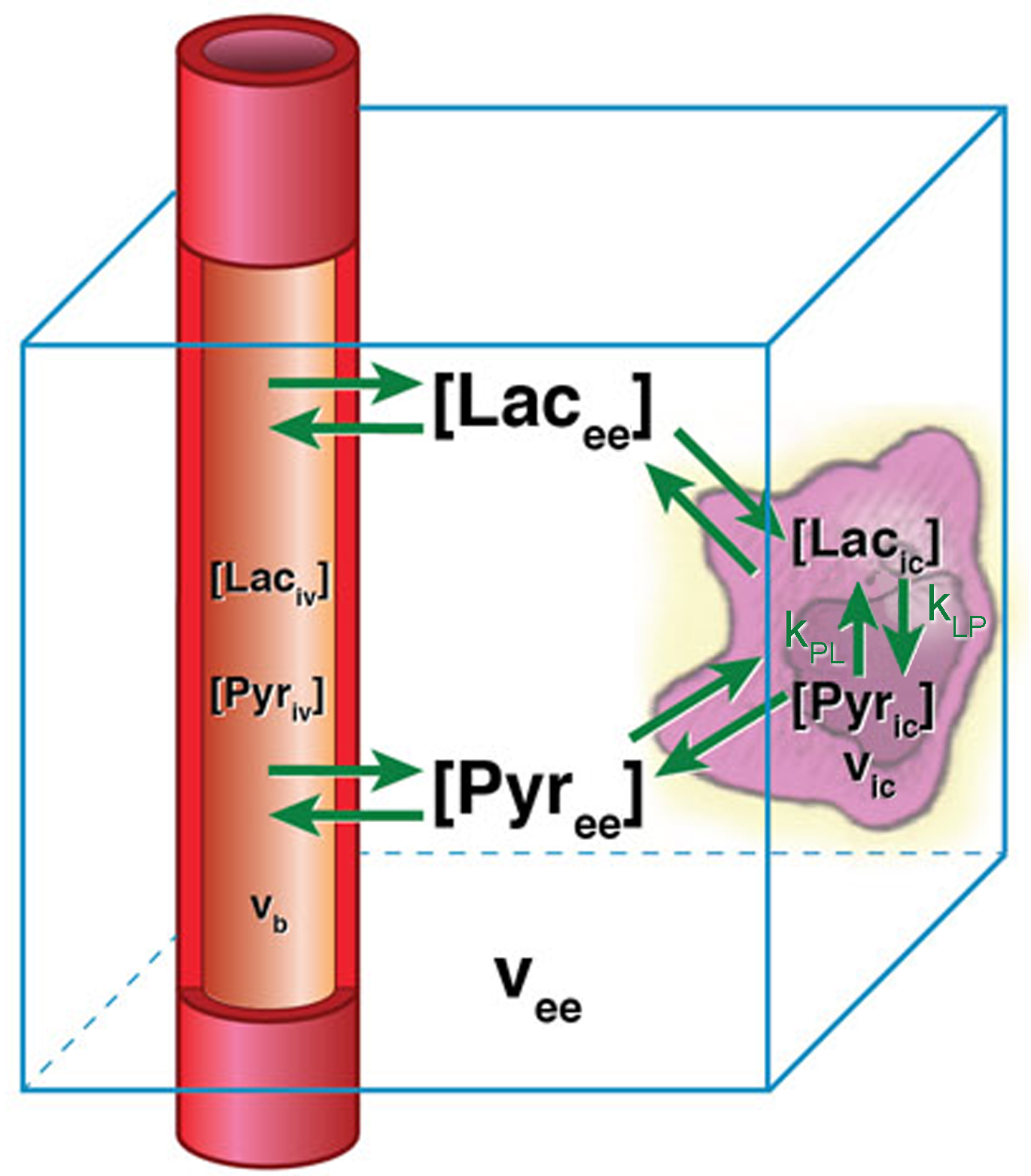
Figure 3: A pharmacokinetic model for HP pyruvate signal evolution comprised of three physical compartments (vascular, extravascular/extracellular, and intracellular) and two chemical pools. HP pyruvate is delivered to tissue via vasculature, but chemical conversion only occurs in the intracellular space. The blue box represents an imaging voxel. This model can be described by the differential equations in Eqs. 11-14. Adapted from Bankson JA, et al. Cancer Research 2015, (18).
Note that all of the transfer and conversion rates in Equations 11-14 have been written as being constant over time, but this will not necessarily reflect the actual enzyme or transport kinetics that may have a Michaelis-Menten relationship (See HP Agents and Biochemical Interactions for more information). \(k_{\text{ecp}}\) and \(k_{\text{ecl}}\) could certainly be written in the form of a Michaelis-Menten relationship to account for potential saturation of monocarboxylate transporters that mediate transport of pyruvate and lactate across the cell membrane. \(k_{\text{PL}}\) and \(k_{\text{LP}}\) could also be expressed as a Michaelis-Menten relationship (15), or as an even more complex relationship that more completely describes the enzymatic activity of lactate dehydrogenase. However, using more detailed models with varying rate constants over time introduces additional unknowns into these equations, and can increase the noise and uncertainty in kinetic analyses – particularly when multiple parameters have a similar effects on signal evolution. In typical HP experiments, using varying rate constants introduces substantial uncertainty and thus constant rate constants are most often used.
Assuming that model parameters can reasonably be assumed to remain constant over an interval of time, we can rewrite this system of equations in matrix notation in the form of \(\dot{\mathbf{x}}(t) = \mathbf{\text{Ax}}(t) + \mathbf{b}(t)\) :
(15)
The diagonal terms (\(\mathbf{\alpha}\)) in \(\mathbf{A}\) reflect attenuation of signal from each volume compartment and chemical pool, and denote the combined parenthesized terms on the right hand sides of equations 11-14. The general analytical solution is found by the variation of parameters approach:
\(\begin{bmatrix} \text{Pyr}_{\text{ee}}(t) \\ \text{Lac}_{\text{ee}}(t) \\ \text{Pyr}_{\text{ic}}(t) \\ \text{Lac}_{\text{ic}}(t) \\ \end{bmatrix} = e^{\mathbf{A}\left( t - t_{0} \right)}\begin{bmatrix} \text{Pyr}_{\text{ee}}(t = t_{0}) \\ \text{Lac}_{\text{ee}}(t = t_{0}) \\ \text{Pyr}_{\text{ic}}(t = t_{0}) \\ \text{Lac}_{\text{ic}}(t = t_{0}) \\ \end{bmatrix} + \frac{k_{\text{ve}}}{v_{\text{ee}}}\int_{t_{0}}^{t}{e^{\mathbf{A}(t - \tau)}\begin{bmatrix} \text{Pyr}_{\text{iv}}(\tau) \\ \text{Lac}_{\text{iv}}(\tau) \\ 0 \\ 0 \\ \end{bmatrix}\text{dτ}}\) (16)
where A is defined as the first matrix on the right hand side of Eq 15. It is convenient to calculate Eq 16 in an iterative fashion over intervals defined by signal excitations in an imaging sequence. Immediately after signal excitation, for example, the observed transverse magnetization will have a \(\sin\left( \theta_{i} \right)\) relationship with the left hand side of Eq 16, given an excitation angle of \(\theta_{i}\) for the ith observation
\(\begin{bmatrix} \text{Pyr}_{ee,xy}(t = t_{\text{obs}}) \\ \text{Lac}_{ee,xy}(t = t_{\text{obs}}) \\ \text{Pyr}_{ic,xy}(t = t_{\text{obs}}) \\ \text{Lac}_{ic,xy}(t = t_{\text{obs}}) \\ \end{bmatrix} = \begin{bmatrix} \text{Pyr}_{\text{ee}}(t_{\text{obs}}) \cdot \sin\theta_{p,i} \\ \text{Lac}_{\text{ee}}(t_{\text{obs}}) \cdot \sin\theta_{l,i} \\ \text{Pyr}_{\text{ic}}(t_{\text{obs}}) \cdot \sin\theta_{p,i} \\ \text{Lac}_{\text{ic}}(t_{\text{obs}}) \cdot \sin\theta_{l,i} \\ \end{bmatrix}\) (17)
The remaining fraction of magnetization in each compartment then becomes the initial value for the next interval (the first term on the right hand side of Eq 16) that will evolve over time until the next excitation pulse while fresh spins accumulate from vasculature according to the last term on the right hand side of the equation.
\(\begin{bmatrix} \text{Pyr}_{\text{ee}}(t = t_{\text{obs}} + TR) \\ \text{Lac}_{\text{ee}}(t = t_{\text{obs}} + TR) \\ \text{Pyr}_{\text{ic}}(t = t_{\text{obs}} + TR) \\ \text{Lac}_{\text{ic}}(t = t_{\text{obs}} + TR) \\ \end{bmatrix} = e^{\mathbf{A \cdot}\text{TR}}\begin{bmatrix} \text{Pyr}_{\text{ee}}(t_{\text{obs}}) \cdot \cos\theta_{p,i} \\ \text{Lac}_{\text{ee}}(t_{\text{obs}}) \cdot \cos\theta_{l,i} \\ \text{Pyr}_{\text{ic}}(t_{\text{obs}}) \cdot \cos\theta_{p,i} \\ \text{Lac}_{\text{ic}}(t_{\text{obs}}) \cdot \cos\theta_{l,i} \\ \end{bmatrix} + \frac{k_{\text{ve}}}{v_{\text{ee}}}\int_{t_{\text{obs}}}^{t_{\text{obs}} + TR}{e^{\mathbf{A}\left( t_{\text{obs}} + TR - \tau \right)}\begin{bmatrix} \text{Pyr}_{\text{iv}}(\tau) \\ \text{Lac}_{\text{iv}}(\tau) \\ 0 \\ 0 \\ \end{bmatrix}\text{dτ}}\) (18)
This approach more accurately reflects excitation losses as periodic events, rather than continuous effects that would be modeled as distributed over time if included in \(R_{Pyr}\) and \(R_{Lac}\) as introduced in Equations 11-14.
The total signal observed will be a combination of the transverse magnetization from each compartment, weighted by their relative volume fractions, which must add to unity:
\(\begin{bmatrix} Pyr(t) \\ Lac(t) \\ \end{bmatrix} = v_{\text{ic}}\begin{bmatrix} \text{Pyr}_{ic,xy}(t) \\ \text{Lac}_{ic,xy}(t) \\ \end{bmatrix} + v_{\text{ee}}\begin{bmatrix} \text{Pyr}_{ee,xy}(t) \\ \text{Lac}_{ee,xy}(t) \\ \end{bmatrix} + v_{b}\begin{bmatrix} \text{Pyr}_{iv,xy}(t) \\ \text{Lac}_{iv,xy}(t) \\ \end{bmatrix}\) (19)
This model includes knowledge of the vascular input function for our imaging agents, and at least eight unique unknowns, even when assuming that rate constants reflecting extravasation (\(k_{\text{ve}}\)) and transport (\(k_{\text{ec}}\)) are equal in both directions for pyruvate and lactate. Many of these are ‘nuisance parameters’ that may not provide much important information, but that must be managed correctly in order to maximize the accuracy and reproducibility of the metabolic information that we seek that is uniquely available from dynamic imaging of HP pyruvate. The more subtle effects of some of these parameters may not be easily captured by HP measurements that are often acquired with relatively low spatial and temporal resolution, and at a modest signal-to-noise ratio.
A slightly simpler pharmacokinetic model can be invoked when appropriate to avoid over-fitting real-world data. If we simplify the model system so that the EES exists in rapid equilibrium with intracellular space via fast diffusion and transport across the cell membrane, then the model needs only account for exchange between two physical pools, as illustrated in Figure 4:
(20)
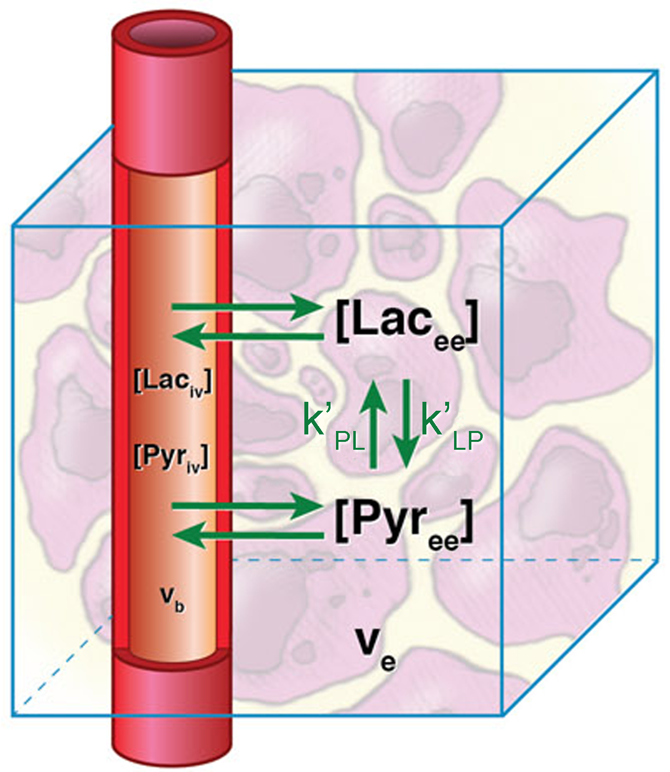
Figure 4: A pharmacokinetic model for HP pyruvate with two physical compartments (vascular, extravascular) and two chemical pools. Here, extravascular space represents a homogeneous mixture of extravascular/extracellular and intracellular space, which were represented separately in the prior 3-compartment PK model illustrated in Fig. 3. Chemical exchange in the extravascular space remains segregated from HP pyruvate in vasculature. The blue box represents an imaging voxel. This model can be described by the differential equations in Eq. 20.
Here we annotate the apparent conversion rate, \(k_{\text{PL}}^{'}\), to differentiate it from the purely intracellular rate constant because in this two-compartment model, \(k_{\text{PL}}^{'}\) relates the HP lactate signal, which is predominantly intracellular, with HP pyruvate that is present in both the intracellular and EES compartments. \(k_{\text{PL}}^{'}\) will be less than \(k_{\text{PL}}\) because it will be affected by transport across the cell membrane, which was specifically accounted for in the three-compartment model, and because this model doesn’t recognize that the substantial pool of HP pyruvate in the EES is not in contact with intracellular enzymes that mediate exchange. The solution to this two-compartment model is similar in form to Eq. 16 but involves fewer equations and model parameters:
\(\begin{bmatrix} \text{Pyr}_{\text{ev}}(t) \\ \text{Lac}_{\text{ev}}(t) \\ \end{bmatrix} = e^{\mathbf{A}\left( t - t_{0} \right)}\begin{bmatrix} \text{Pyr}_{\text{ev}}(t = t_{0}) \\ \text{Lac}_{\text{ev}}(t = t_{0}) \\ \end{bmatrix} + \frac{k_{\text{ve}}}{v_{e}}\int_{t_{0}}^{t}{e^{\mathbf{A}(t - \tau)}\begin{bmatrix} \text{Pyr}_{\text{iv}}(\tau) \\ \text{Lac}_{\text{iv}}(\tau) \\ \end{bmatrix}\text{dτ}}\) (21)
Here, the matrix A is redefined as the first matrix on the right hand side of Eq. 20.
The matrix exponentials in Equations 17 and 20 can make it difficult to visualize what these models predict without running simulations. However, a few additional assumptions can simplify the system enough to write the solution in a much more digestible form. If we assume that (1) no hyperpolarized lactate is brought into tissue through vasculature (\(\text{Lac}_{\text{iv}}(t) = 0\)); and (2) that the “reverse” conversion of HP lactate to pyruvate is negligibly small (\(k_{\text{LP}}^{'} = 0\)); and (3) that observations begin before any hyperpolarized imaging agents are present in the system (\(\text{Pyr}_{\text{ev}}(t = 0) = \text{Lac}_{\text{ev}}(t = 0) = 0)\), then Eq. 21 becomes a much more familiar expression:
\(\text{Pyr}(t) = k_{\text{ve}}\int_{t_{0}}^{t}{e^{\mathbf{-}\alpha_{P,e}(t - \tau)}\text{Pyr}_{\text{iv}}(\tau)\text{dτ}} + v_{b}\text{Pyr}_{\text{iv}}(t)\) (22)
\(\text{Lac}(t) = k_{\text{PL}}^{'}\int_{t_{0}}^{t}{e^{\mathbf{-}\alpha_{L,e}(t - \tau)}\text{Pyr}_{\text{ev}}(\tau)\text{dτ}}\)
\(= \frac{k_{\text{ve}}k_{\text{PL}}^{'}}{\alpha_{P,e}\mathbf{-}\alpha_{L,e}}\int_{t_{0}}^{t}{\left( e^{\mathbf{-}\alpha_{L,e}(t - \tau)} - e^{\mathbf{-}\alpha_{P,e}(t - \tau)} \right)\text{Pyr}_{\text{iv}}(\tau)\text{dτ}}\) (23)
Equation 22 closely resembles the well-known extended Tofts model for extravasation of Gd-based contrast agents during a dynamic, contrast-enhanced (DCE-) MRI measurement (20). Pyruvate in the extravascular space grows according to \(k_{\text{ve}}\), the rate constant for extravasation from vascular to extravascular space, and it is reduced over time by an attenuation term that includes chemical conversion to lactate, loss back into vascular space, and attenuation of the HP signal due to spin-lattice relaxation, excitation losses and/or conversion to other chemical endpoints. Equation 23 says that HP lactate in the extravascular space grows from HP pyruvate in that volume compartment according to \(k_{\text{PL}}^{'}\), the apparent rate constant for conversion of HP pyruvate into lactate, and that the HP lactate signal is reduced by an attenuation term that includes loss into vascular space and spin-lattice relaxation. The second form of Eq. 23 helps to illustrate that the HP lactate signal also depends heavily on the rate at which HP pyruvate extravasates from vasculature. Fortunately, vasculature in many cancers is torturous and malformed, leading to rapid extravasation of contrast agents, including HP pyruvate.
Both of the presented PK models (Figs. 3 and 4) segregate HP pyruvate in vasculature from HP pyruvate that is in contact with the enzymes that mediate chemical conversion, which are known to be present primarily in cytosol. Both require information about the vascular input function for HP pyruvate. Accurate measurement of the vascular input function is known to be a notoriously difficult task in DCE-MRI studies, where flow-related enhancement, vessel orientation, and partial volume effects can confound estimation of Gd content in vasculature. Although direct observation of HP pyruvate and lactate in an HP MRI measurement is not as sensitive to flow enhancement, consistent estimation of the HP pyruvate vascular input function may still prove challenging in many cases.
When information about the vascular input function is unavailable or unreliable for a set of measurements, the kinetic models described by Equations 16 and 21-23 cannot be used. In that case, the relationship between HP pyruvate and lactate can be written as a simple precursor-product relationship:
\(\frac{\partial Lac(t)}{\partial t} = k_{\text{PL}}^{''}\text{Pyr}(t) - R_{\text{Lac}}Lac(t)\) (22)
Which yields
\(\text{Lac}(t) = e^{\mathbf{-}R_{\text{Lac}}\left( t - t_{0} \right)}\text{Lac}\left( t = t_{0} \right) + k_{\text{PL}}^{''}\int_{t_{0}}^{t}{e^{\mathbf{-}R_{\text{Lac}}(t - \tau)}\text{Pyr}(\tau)\text{dτ}}\) (23)
This equation relates the HP lactate signal in each voxel to the total HP pyruvate signal, implying that all observed pyruvate is in contact with enzymes that mediate chemical conversion (See Fig. 5). The precursor-product relationship has been used extensively, including for early in vivo HP studies (35,36). However, over-estimation of the amount of pyruvate in contact with these enzymes can lead to under-estimation of metabolic activity in tumor cells. Here again, \(k_{\text{PL}}^{''}\) should be differentiated from previous rate constants because it will be affected by additional confounds associated with vasculature. \(k_{\text{PL}}^{''}\) will be less than \(k_{\text{PL}}^{'}\) because the HP pyruvate signal from all compartments is considered against HP lactate which can only arise after extravasation, transport, and chemical conversion (See Fig. 6). However, the simplicity of this relationship is very appealing since quantification of \(k_{\text{PL}}^{''}\ \) is not obfuscated by nuisance parameters other than the spin-lattice relaxation rate of HP lactate – which can be designed to be a small effect compared to controllable excitation losses. Finally, if vascular characteristics can be reasonably assumed, or demonstrated through measurements, to be stable across multiple separate measurements, then any changes that are observed in \(k_{\text{PL}}^{''}\ \) using this model should be attributable to changes in metabolic activity rather than reflective of confounding changes in vascular factors that impact HP MRI signal evolution.
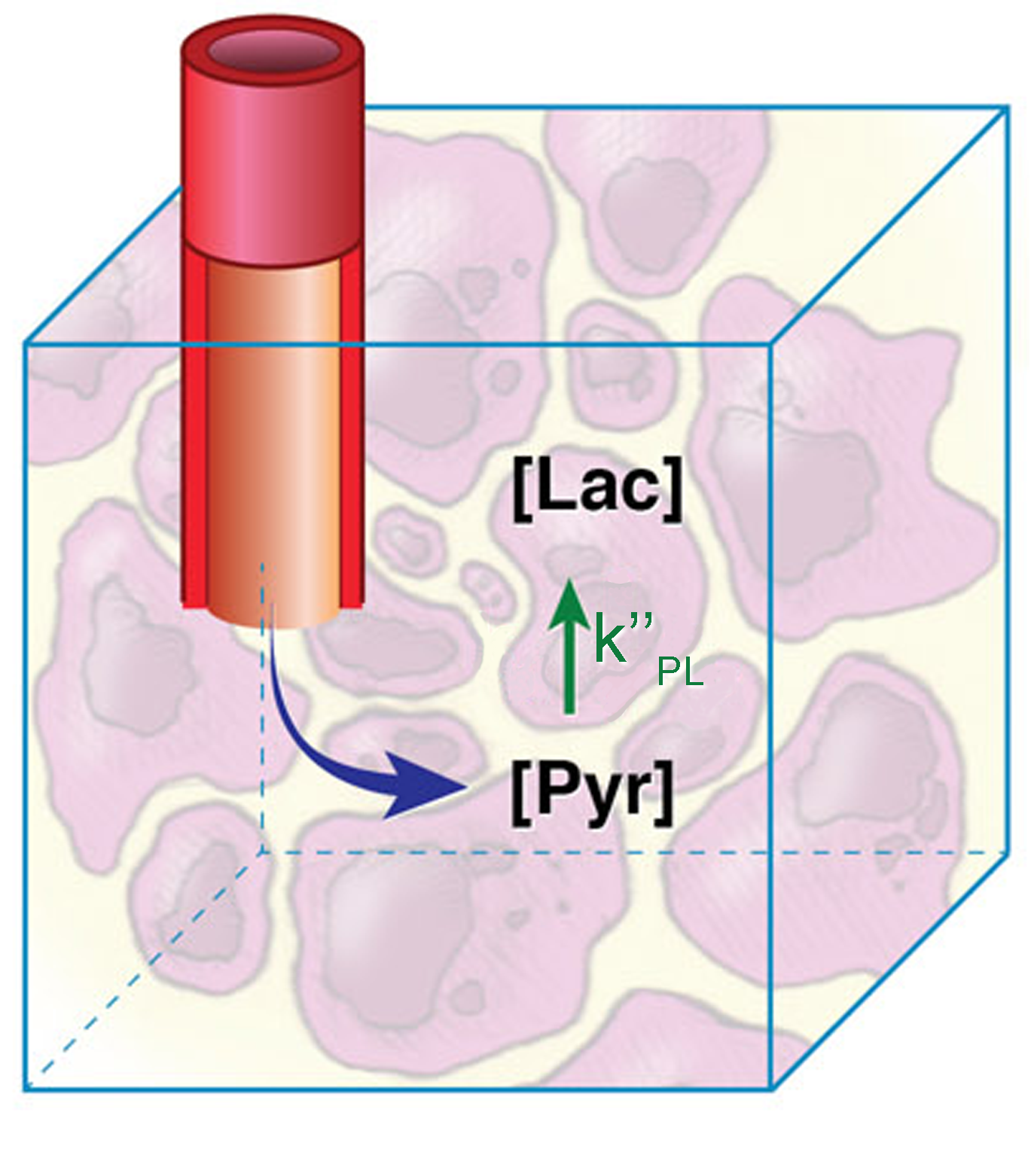
Figure 5: Precursor-product model for HP pyruvate in a single physical compartment. All observed signal is assumed to be in contact with enzymes that mediate exchange. The blue cube represents an imaging voxel. This model is described in Eq. 23.
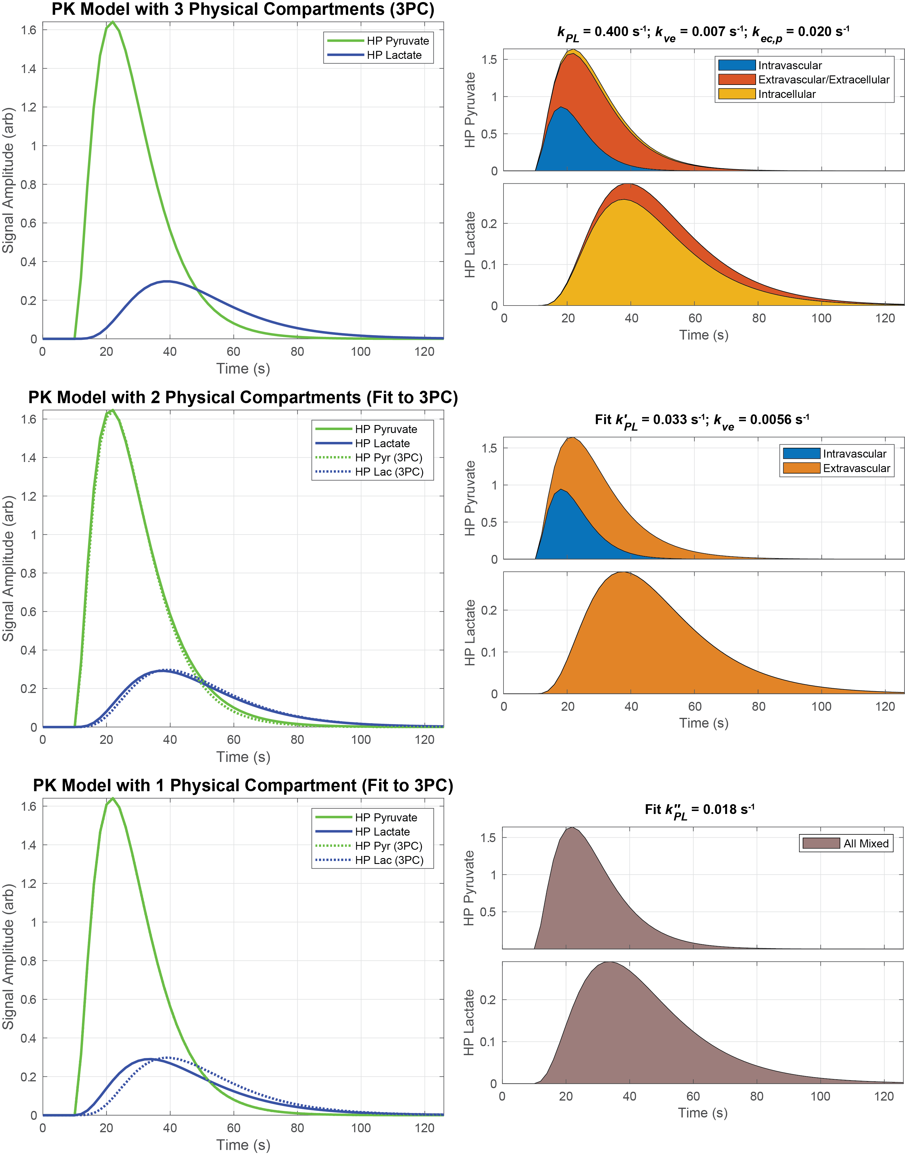
Figure 6: Fitting data from a three physical compartment (3PC) simulation to PK models with one, two, and three physical compartments. Top: Simulation of HP pyruvate and lactate with physiologically reasonable (but not definitive) model parameters (3PC model from Fig. 3). Note that rapid intracellular conversion of pyruvate to lactate results in low pyruvate and high lactate within that compartment. Middle: the two-compartment model (Fig. 4) was fit to the overall signal curve generated from the three-compartment model, assuming that the pyruvate vascular input function and fractional blood volume fraction were known and the same as used in simulation. Bottom: the overall signal curve generated from the three-compartment model was analyzed using the one-compartment (precursor-product) model (Fig. 5). The slight temporal shift in the lactate curve is due to simplifying assumptions that eliminate biological hurdles that act to delay chemical conversion. Note that the apparent reaction rate is progressively lower as the model simplified: \(k_{\text{PL}} > k_{\text{PL}}^{'} > k_{\text{PL}}^{''}\) .
Choosing a Model#
Selection of the most appropriate pharmacokinetic model for analysis of HP MRI data requires careful consideration of study goals and the quality and characteristics of the underlying data. Higher order models reduce bias that may be imparted by confounding factors that affect signal evolution, and permit estimation of parameters that aren’t available in simpler models. For example, lactate efflux has been shown to be a significant factor in several tumor types, particularly renal tumors (21), and parameters that reflect efflux can be captured by PK models with two or three physical compartments to provide an additional biomarker of tumor aggressiveness (17). As a contrary example, data from glioblastoma cells was shown to be best fit by a pre-cursor-product model with a single physical compartment (22).
Higher order models can also lead to increased uncertainty in the estimation of model parameters. PK models with more than one physical compartment require estimation of an arterial input function, and the quality of that estimate can affect the accuracy and reproducibility of quantitative metabolic analyses(23). Data must be acquired with sufficient SNR to detect subtle differences in the shape of the signal curves. Thus it is important to find the appropriate level of model complexity that can be supported by the data that is available. Tools such as Akaike’s Information Criterion (AIC), which rewards a good fit between data and candidate models and penalizes the use of additional model parameters, can provide a useful framework for model selection (24). AIC has been used to select the 2-compartment model as the appropriate compromise between simplicity and complexity when examining slice- and coil-localized dynamic spectroscopic data from a variety of murine models of cancer (18). However, more (or less) complex models may be more appropriate when working with data that has higher (or lower) SNR, better (or worse) spatiotemporal resolution, or acquired from human subjects or other disease sites.
Fitting Algorithms#
The final step in implementing a PK model for HP data analysis is to choose an appropriate algorithm for data fitting. This is commonly achieved by solving a non-linear least-squares curve fitting problem, for example with the ‘lsqnonlin()’ function in MATLAB. In this approach, the sum of the squared residuals between the data and PK model with certain parameters is minimized. A least-squares approach is optimal when the noise is Gaussian, but can have biased estimates if magnitude data is used because it has a Rician noise distribution that is especially problematic for low SNR (see ‘Data Extraction’ above). For the PK models and typical HP data, this is often a non-convex problem, meaning the fitting can be very sensitive to the initial guess of the model parameters. Thus the initial guess in the fitting should be carefully chosen. Repeated fits that explore a defined parameter space via grid sampling or by random selection of seed points can help reduce the likelihood of fitting to local minima.
Fitting is also typically done in the time domain, but can also be applied in other domains. Frequency domain fitting, achieved by applying the Laplace or Fourier transform to the data, has advantages of fitting to more sparse data (25) and can also estimate a distribution or multiple rate constants (26).
For precursor-product models, fitting can also be performed in an “inputless” manner, where only the metabolic products data is fit to the model while the substrate data is taken as ground truth and not fit to any curve (25, 30). This approach requires no estimate of the vascular input function and is thus relatively robust due to its simplicity.
Model-free Metrics#
Kinetic models are conceptually appealing in that they attempt to characterize relationships between biological compartments and biochemical processes and improve the specificity to which potential changes could be attributed. Furthermore, they can be potentially invariant of many experimental conditions and confounds since they are primarily dependent on the HP agent behavior, which allows for broader comparisons across experiments. However, they have several disadvantages: simpler kinetic models are often favored due to practical limitations of the HP experiment; other information that may be difficult to obtain (e.g. compartment volumes, vascular input functions) is needed for more complex models; the results are susceptible to errors when there is mismatch between the model and the data; and the fact that there can be considerable instabilities in model fitting, particularly with more complex models, and they require more sophisticated implementations than many of the model-free alternatives described next. For these reasons, model-free metrics of metabolic conversion, several of which are illustrated in Fig. 7, have been developed and are a popular alternative to kinetic models.
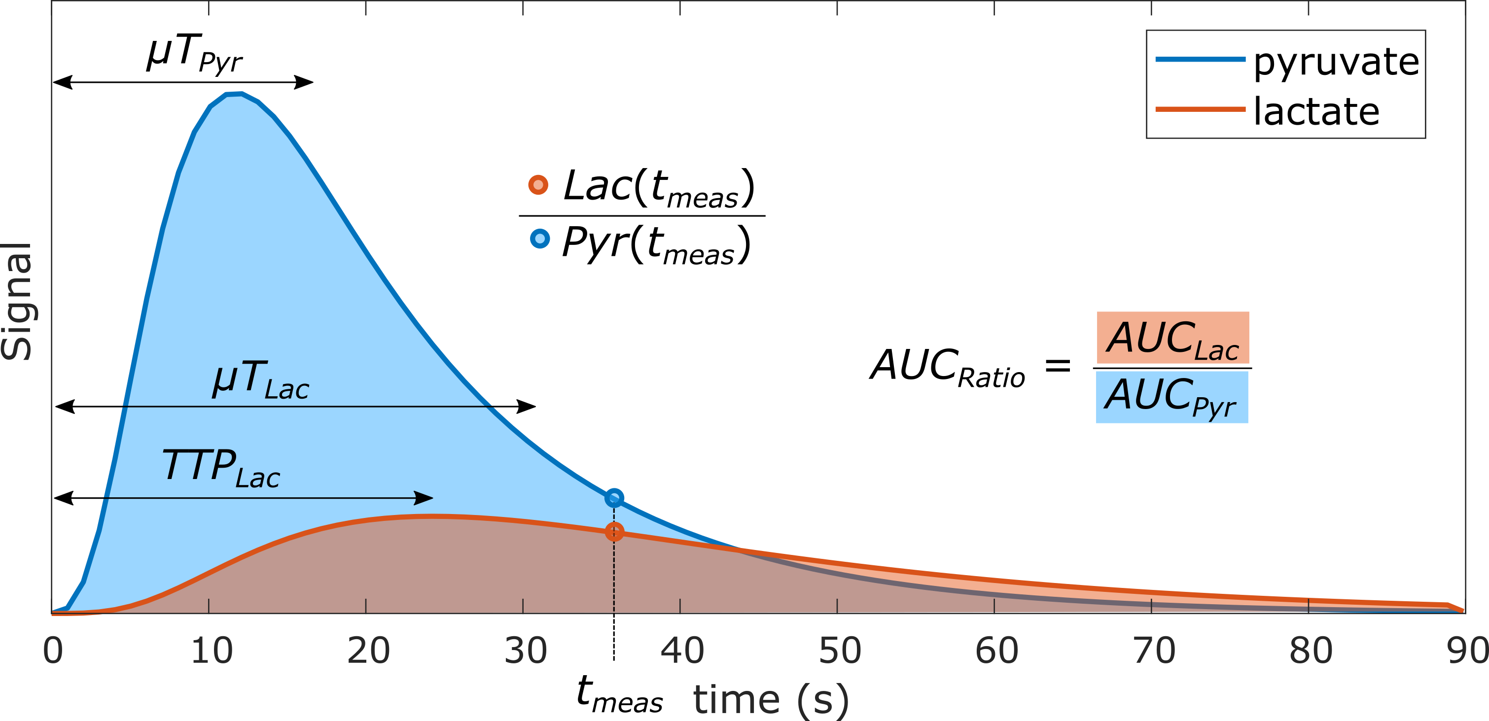
Figure 7: Illustration of several model-free metrics that can be used for HP data. These include the lactate-to-pyruvate ratio at a single time-point (\(\mathrm{Lac}(t_\mathrm{meas})/\mathrm{Pyr}(t_\mathrm{meas})\)), the area-under-curve (AUC) ratio (\(\mathrm{AUC}_\mathrm{ratio}\)), lactate time-to-peak (\(\mathrm{TTP}_\mathrm{Lac}\)), and the mean time (\(\mu T\)) for a metabolite. Inspired by Daniels CJ, et al. \textit{NMR Biomed} 2016 (27) .
Metabolite Ratios#
The most common model-free metrics used in quantification of HP data are metabolite ratios in which the denominator is the substrate or total 13C signal. These “Ratiometric” approaches have several advantages: first and foremost, they provide a metric reflecting metabolic conversion that is straightforward to compute; also, they include inherent normalization such that they are largely invariant to the amount of polarization, RF coil sensitivities, and amount of agent delivered.
Single time-point: In the simplest form, metabolite ratios can be computed from data at a single time-point, as illustrated in Fig. 7 by \(\mathrm{Lac}(t_\mathrm{meas})/\mathrm{Pyr}(t_\mathrm{meas})\). However, this approach is sensitive to the timing of this single time-point because of the typically rapid rates of bolus delivery, metabolic conversion, and signal decay, which results in signals and the ratio between them varying continuously throughout their observable lifetime. This can be partially addressed by selecting a stable and reproducible measurement time relative to the bolus in a dynamic acquisition (28), if one can be identified.
Area-under-curve (AUC): The more robust approach is to perform a dynamic acquisition and compute the area-under-curve (AUC) ratio from the metabolite time courses, illustrated in Fig. 7 by \(\mathrm{AUC}_{\mathrm{ratio}}\). This approach has been shown to be proportional to the metabolic conversion rate under certain conditions (37). With assumptions that the acquisition covers the entire dynamic acquisition, including the bolus delivery, and an underlying precursor-product kinetic model (Eq. 23, Fig. 5), the AUC ratio between lactate and pyruvate is:
\(\text{AU}C_{\text{ratio}} = \frac{\text{AU}C_{\text{Lac}}}{\text{AU}C_{\text{Pyr}}} = \frac{k_{\text{PL}}^{''}}{R_{\text{Lac}} + k_{\text{LP}}^{''}}.\) (24)
This relationship trivially extends to other HP agents with precursor-product conversion processes, and also is valid when the substrate is converted into multiple products (e.g. [1-13C]pyruvate to [1-13C]alanine and 13C-bicarbonate).
This proportionality holds for all flip angle schemes which do not change over time, including metabolite-specific flip angles (See Hyperpolarized Acquistion Methods). It does, however, depend on the flip angles used (here, \(R_{\text{Lac}}\) includes excitation losses); the AUC ratio cannot be compared across studies that use different flip angles without additional corrections. The proportionality between the AUC ratio and \(k_{\text{PL}}\) breaks down when flip angles vary over time if there are any variations in vasculature or bolus characteristics.
Direct versus Differential conversion: A metric of direct metabolic conversion can be calculated by taking a direct or AUC ratio between the product and substrate, e.g. lactate/pyruvate, as described above. In some cases, the differential metabolic conversion is informative, for example when studying glucose metabolism versus oxidative metabolism. For this case, the signal amplitude or AUC ratio between products (eg, 13C-bicarbonate and [1-13C]lactate, following [1-13C]pyruvate injection) will reflect differences in metabolic preference. Because both products depend on substrate delivery in the same way, differential conversion may be relatively insensitive to vascular or bolus characteristics.
Normalized metabolic product amplitudes#
Normalized metabolic product signal amplitudes, e.g. \(\mathrm{Lac}(t_\mathrm{meas})\) or \(\mathrm{AUC}_{\mathrm{Lac}}\), have also been successfully used as a measure of metabolic conversion. Most notably, in the human brain, lactate signal amplitudes have been normalized to the mean across all brain regions in a subject for ‘lactate topography’ (29). Most other metrics have some inherent normalization to the substrate, e.g. pyruvate, which makes them insensitive to variations in polarization and RF coil profiles, and provides some normalization to substrate delivery. Using downstream metabolic product signals on their own has potential to eliminate some partial volume effects, like substrate signals in major vasculature that may not be metabolically accessible. Also, in cases where cellular transport and/or the enzyme-mediated conversion is saturated (sometimes this is done by design, see HP Experimental Methods: Cells and Animals), variations in substrate dose above a certain level will result in the same product signal, resulting in erroneous variations of metrics normalized by the substrate. But these potential benefits are speculative, and normalizing to substrate amplitudes has many benefits as well. Furthermore, normalizing product signal amplitudes must account for non-trivial variations in polarization and RF coil sensitivities.
Dynamic metrics#
Since the metabolic conversion is a dynamic process, metrics based on the temporal characteristics of the data can also be used. One proposed is the lactate time-to-peak (\(\mathrm{TTP}_{\mathrm{Lac}}\)), which has been shown to be inversely proportional to \(k_{\text{PL}}^{''}\). However, this metric performs poorly with low SNR (Supplemental Data in (30)).
Another proposed dynamic metric is the “Mean Time”, calculated as the center of mass of the dynamic signal curves (30, 31). This is illustrated in Fig. 7 as µT, and notably is later in time than the peak signal. For the substrate, the mean time can be used as a measure of the arrival time. For metabolic products this metric is similar to the TTP but slightly more robust to SNR (REF). The metric also reflects additional effects such as variations in \(T_1\) relaxation rates, and flow in and out of the tissue.
Evaluation of Metabolism Metrics#
It is very challenging to evaluate the accuracy of HP metabolism metrics in vivo because it is nearly impossible to have a ground truth values and the apparent rate constants can be influenced by a combination of perfusion/delivery, cellular uptake, pool sizes, intracellular transport (e.g. into mitochondria), enzymatic conversion, efflux out of cells, and out-flow, and compartmental \(T_1\) differences (32). Arguably, ground truth in HP experiments may only be accessible in highly controlled systems (e.g. cell systems, see HP Experimental Methods: Cells and Animals).
Given this limitation, simulations can be used very effectively to provide insight into evaluation of HP metabolism metrics. Simulation parameters to evaluate should include key HP experimental variables such the conversion rates, relaxation rates, noise level, acquisition strategy (flip angles, timing), bolus and perfusion characteristics, and flip angle accuracy.
Monte Carlo simulations, in which a signal is analyzed many times in the presence of unique added noise, can be used to characterize the response of metrics, both in terms of accuracy and precision (26, 30, 33). The PK model and model parameters that are used to generate synthetic signal can have significant impact on the outcome of these kinds of analyses, and must be considered carefully (33). Figure 8 shows a Monte Carlo simulation using a precursor-product kinetic model comparing an “inputless” fitting method (30)(Eq. 23) with fixed relaxation rates, inputless fitting including \(T_{1,\mathrm{Lac}}\) fitting, and lactate to pyruvate AUC ratio, all for three different flip angle schemes. From these simulations, we can see that the relative accuracy (indicated by error bars) is similar between the inputless fitting with fixed rates and the AUC ratio, while fitting \(T_{1,\mathrm{Lac}}\) increases expected error. They show that using metabolite-specific flip angles leads to expected improvements in precision over the constant uniform flip angles as well as the variable flip angle scheme chosen. Finally, they also show that the AUC ratio varies depending on the flip angle strategy.
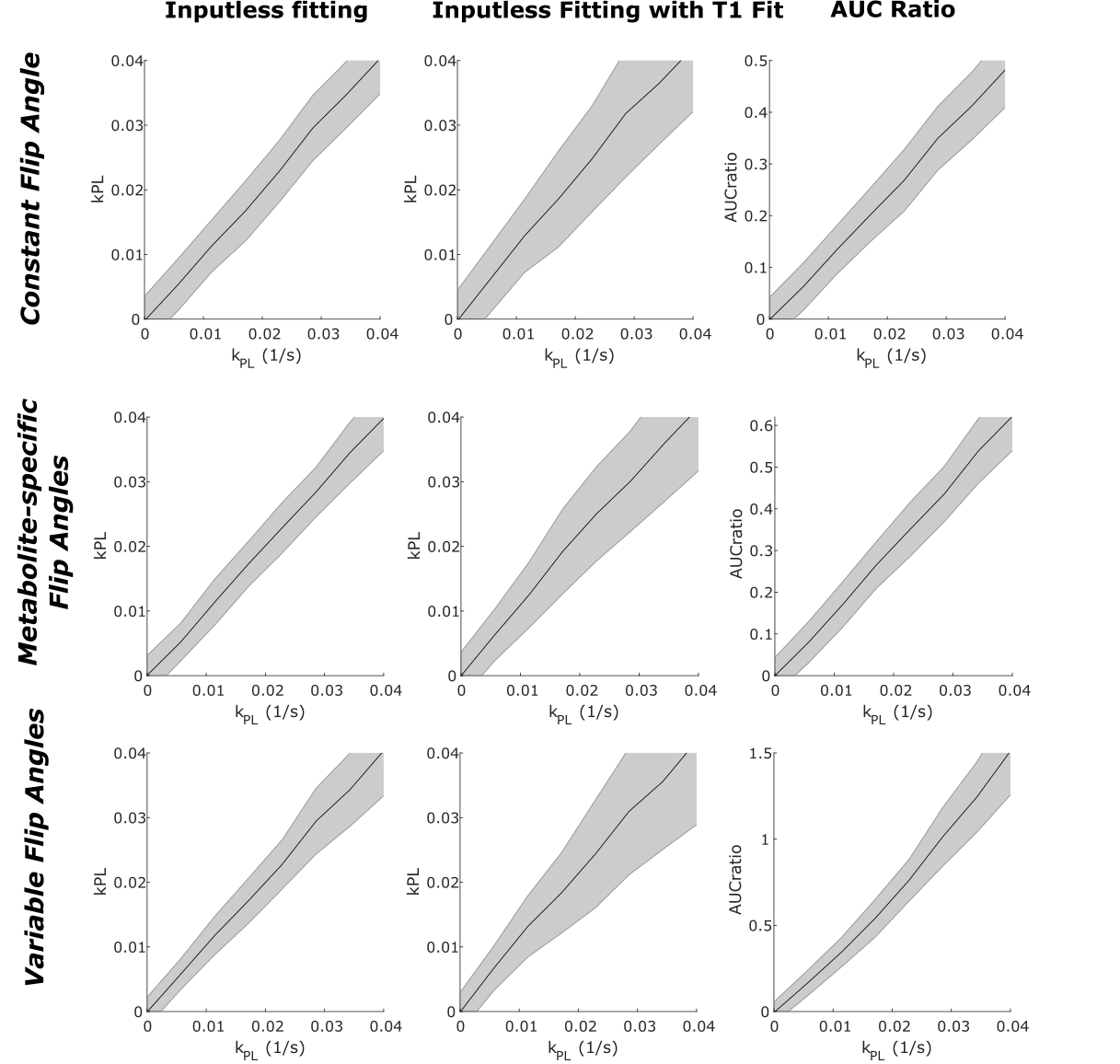
Figure 8: Simulation comparison of HP metabolism metrics as function of \(k_{\text{PL}}\) for different flip angle strategies. A Monte Carlo simulation of a precursor-product model (Fig. 5) was used to show their response to noisy data, where the solid lines represent the mean of the metric and the shaded regions represent the standard deviation of the fitting across different noise in the test data. The simulations used nominal parameters of \(T_{1,\mathrm{Lac}} = 25 \, \mathrm{s}\), \(T_{1,\mathrm{Pyr}} = 30 \, \mathrm{s}\), \(T_{\mathrm{arrival}} = 4 \, \mathrm{s}\), and \(T_{\mathrm{bolus}} = 8 \, \mathrm{s}\), with experimental parameters of \(TR = 3 \, \mathrm{s}\), over 16 time points. The “Constant flip angle” was 25-degrees, “Metabolite-specific flip angles” were 20-degrees (pyruvate) and 30-degrees (lactate), and “Variable flip angles” using a T1-effective scheme for pyruvate with \(T_{1,\mathrm{effective}} = 20 \, \mathrm{s}\) and a maximum SNR scheme for lactate with \(T_{1,\mathrm{Lac}} = 25 \, \mathrm{s}\).
Figure 9 shows additional Monte Carlo simulation results using the same precursor-product kinetic model, but presented in terms of relative \(k_{\text{PL}}^{''}\) error, and with simulations across a range of potential experimental variability. The purpose of this simulation is to evaluate the response of a given metric, fitting approach, or flip angle scheme in response to variable conditions. The experimental ranges for \(k_{\text{PL}}\), noise standard deviation (σ), bolus characteristics (\(T_{\text{arrival}}\), \(T_{\text{bolus}}\)), relaxation rates, “\(B_1\) error” (unknown changes in \(B_1\) field), and “\(B_1\) change” (known changes in \(B_1\) field) are based on typical in vivo results (30). These results show that the AUC ratio and inputless fitting with fixed relaxation rates perform comparably, except when the bolus arrival is not captured (\(T_{\text{arrival}} > 0\)), in which case the AUC ratio deviates from the expected nominal value. Both of these methods suffer from bias if \(T_{1,\text{Lac}}\) is not known or in the presence of unknown \(B_{1}\) errors. Fitting for \(T_{1,\text{Lac}}\) leads to worse precision, but more accurate response in the presence of unknown \(T_{1,\text{Lac}}\) and \(B_{1}\) errors.

Figure 9: Simulation comparison of HP metabolism relative metric accuracy and precision in response to variations in experimental parameters of \(k_{\text{PL}}\), noise level (\(\sigma\)), bolus arrival time (\(T_{\text{arrival}}\)), bolus duration (\(T_{\text{bolus}}\)), metabolite relaxation rates, flip angle errors (”\(B_{1}\) error”), and flip angle differences (”\(B_{1}\) change” i.e. known changes in flip angle). A Monte Carlo simulation of a precursor-product model (Fig. 5) was used to show their response to noisy data, where the solid lines represent the mean of the metric and the dashed lines represent the standard deviation across different noise in the test data. The signal and noise is scaled such that the total available magnetization provided equals 1. In other words, the maximum signal would be 1 if it were all excited with a single 90-degree RF pulse. The simulations used nominal parameters of \(T_{1,\text{Lac}} = 25 \, \mathrm{s}\), \(T_{1,\text{Pyr}} = 30 \, \mathrm{s}\), \(T_{\text{arrival}} = 4 \, \mathrm{s}\), and \(T_{\text{bolus}} = 8 \, \mathrm{s}\), with experimental parameters of \(TR = 3 \, \mathrm{s}\), 16 time points, and metabolite-specific flip angles of 20-degrees (pyruvate) and 30-degrees (lactate). This type of simulation allows for comparisons of robustness between different HP metrics. (Adapted from Larson PEZ, et al. NMR in Biomedicine 2018, (30))
Summary#
Specialized data extraction, visualization, and analysis methods are required due to the unique characteristics of HP signals, including high dimensionality, unrecoverable signal decay, metabolic conversion, and bolus and perfusion effects. Data extraction can be performed with methods borrowed from conventional MRI and MRS. Data visualization requires co-registration with anatomical 1H MRI and support for up to 5-dimensional (3 spatial, 1 spectral, 1 temporal) data. Analysis to extract apparent metabolic rate constants can be performed using pharmacokinetic models, which can include effects of metabolic conversion, perfusion, and cellular transport, although often a simple precursor-product model is used. There are also model-free metrics that can accurately reflect metabolic rates under certain conditions, including the AUC ratio. While the examples in this chapter focused on HP pyruvate as a substrate converting to lactate, the models presented can be extended to other metabolic pathways and other HP agents. Evaluation of kinetic models and analysis metrics relies largely on simulations given the challenges of acquired ground truth data in vitro or in vivo.
Many of the kinetic models and metrics described, as well as code to generate the simulation results, are available as part of the hyperpolarized-mri-toolbox (LarsonLab/hyperpolarized-mri-toolbox ) (38).
References#
Provencher SW. Estimation of metabolite concentrations from localized in vivo proton NMR spectra. Magn Reson Med 30(6):672-9, 1993.
Gudbjartsson H, Patz S. The Rician distribution of noisy MRI data. Magn Reson Med 34(6):910-4, 1995. PMCID: PMC2254141.
Henkelman RM. Measurement of signal intensities in the presence of noise in MR images. Med Phys 12(2):232-3, 1985.
Bernstein MA, Thomasson DM, Perman WH. Improved detectability in low signal-to-noise ratio magnetic resonance images by means of a phase-corrected real reconstruction. Med Phys 16(5):813-7, 1989.
Maidens J, Gordon JW, Arcak M, Larson PEZ. Optimizing Flip Angles for Metabolic Rate Estimation in Hyperpolarized Carbon-13 MRI. IEEE Transactions on Medical Imaging 35(11):2403-12, 2016. PMCID: PMC5134417.
Miller AJ, Joseph PM. The use of power images to perform quantitative analysis on low SNR MR images. Magn Reson Imaging 11(7):1051-6, 1993.
Crane JC, Olson MP, Nelson SJ. SIVIC: Open-Source, Standards-Based Software for DICOM MR Spectroscopy Workflows. Int J Biomed Imaging 2013:169526, 2013. PMCID: PMC3732592.
SIVIC. [cited 2018 August 29]. https://sourceforge.net/projects/sivic
OsiriX. [cited 2018 August 29]. https://www.osirix-viewer.com
HOROS. [cited 2018 August 29]. https://horosproject.org
JMRUI. [cited 2018 Aug 29]. http://www.jmrui.eu/welcome-to-the-new-mrui-website
TARQUIN. [cited 2018 Aug 29]. http://tarquin.sourceforge.net
Wilson M, Reynolds G, Kauppinen RA, Arvanitis TN, Peet AC. A constrained least-squares approach to the automated quantitation of in vivo (1)H magnetic resonance spectroscopy data. Magn Reson Med 65(1):1-12, 2011.
Crane JC, Gordon JW, Chen H-Y, Autry AW, Li Y, Olson MP, Kurhanewicz J, Vigneron DB, Larson PEZ, Xu D. Hyperpolarized 13C MRI data acquisition and analysis in prostate and brain at University of California, San Francisco. NMR in Biomedicine n/a(n/a):e4280, 2020. PMCID: PMC7501204.
Witney TH, Kettunen MI, Brindle KM. Kinetic modeling of hyperpolarized 13C label exchange between pyruvate and lactate in tumor cells. J Biol Chem 286(28):24572-80, 2011. PMCID: PMC3137032.
Walker CM, Lee J, Ramirez MS, Schellingerhout D, Millward S, Bankson JA. A catalyzing phantom for reproducible dynamic conversion of hyperpolarized [1-¹³C]-pyruvate. PLoS One 8(8):e71274, 2013. PMCID: PMC3744565.
Ahamed F, Van Criekinge M, Wang ZJ, Kurhanewicz J, Larson P, Sriram R. Modeling hyperpolarized lactate signal dynamics in cells, patient-derived tissue slice cultures and murine models. NMR in Biomedicine 34(3):e4467, 2021.
Bankson JA, Walker CM, Ramirez MS, Stefan W, Fuentes D, Merritt ME, Lee J, Sandulache VC, Chen Y, Phan L, Chou PC, Rao A, Yeung SC, Lee MH, Schellingerhout D, Conrad CA, Malloy C, Sherry AD, Lai SY, Hazle JD. Kinetic modeling and constrained reconstruction of hyperpolarized [1-13C]-pyruvate offers improved metabolic imaging of tumors. Cancer Res 75(22):4708-17, 2015. PMCID: PMC4651725.
Fala M, Somai V, Dannhorn A, Hamm G, Gibson K, Couturier DL, Hesketh R, Wright AJ, Takats Z, Bunch J, Barry ST, Goodwin RJA, Brindle KM. Comparison of (13) C MRI of hyperpolarized [1-(13) C]pyruvate and lactate with the corresponding mass spectrometry images in a murine lymphoma model. Magn Reson Med 85(6):3027-35, 2021.
Tofts PS. Modeling tracer kinetics in dynamic Gd-DTPA MR imaging. J Magn Reson Imaging 7(1):91-101, 1997.
Keshari KR, Sriram R, Koelsch BL, Van Criekinge M, Wilson DM, Kurhanewicz J, Wang ZJ. Hyperpolarized 13C-pyruvate magnetic resonance reveals rapid lactate export in metastatic renal cell carcinomas. Cancer Res 73(2):529-38, 2013. PMCID: PMC3548990.
Harrison C, Yang C, Jindal A, DeBerardinis RJ, Hooshyar MA, Merritt M, Dean Sherry A, Malloy CR. Comparison of kinetic models for analysis of pyruvate-to-lactate exchange by hyperpolarized 13 C NMR. NMR Biomed 25(11):1286-94, 2012. PMCID: PMC3469722.
Sun CY, Walker CM, Michel KA, Venkatesan AM, Lai SY, Bankson JA. Influence of parameter accuracy on pharmacokinetic analysis of hyperpolarized pyruvate. Magn Reson Med 79(6):3239-48, 2018. PMCID: PMC5843516.
Burnham KP, Anderson DR. Model selection and multimodel inference: a practical information-theoretic approach. 2nd ed. New York, NY: Springer-Verlag New York Inc; 2002.
Khegai O, Schulte RF, Janich MA, Menzel MI, Farrell E, Otto AM, Ardenkjaer-Larsen JH, Glaser SJ, Haase A, Schwaiger M, Wiesinger F. Apparent rate constant mapping using hyperpolarized [1-(13)C]pyruvate. NMR Biomed 27(10):1256-65, 2014.
Mariotti E, Veronese M, Dunn JT, Southworth R, Eykyn TR. Kinetic analysis of hyperpolarized data with minimum a priori knowledge: Hybrid maximum entropy and nonlinear least squares method (MEM/NLS). Magn Reson Med 73(6):2332-42, 2015.
Daniels CJ, McLean MA, Schulte RF, Robb FJ, Gill AB, McGlashan N, Graves MJ, Schwaiger M, Lomas DJ, Brindle KM, Gallagher FA. A comparison of quantitative methods for clinical imaging with hyperpolarized 13C-pyruvate. NMR in Biomedicine 29(4):387-99, 2016. PMCID: PMC4833181.
Granlund KL, Tee SS, Vargas HA, Lyashchenko SK, Reznik E, Fine S, Laudone V, Eastham JA, Touijer KA, Reuter VE, Gonen M, Sosa RE, Nicholson D, Guo YW, Chen AP, Tropp J, Robb F, Hricak H, Keshari KR. Hyperpolarized MRI of Human Prostate Cancer Reveals Increased Lactate with Tumor Grade Driven by Monocarboxylate Transporter 1. Cell Metab 31(1):105-14 e3, 2020. PMCID: PMC6949382.
Lee CY, Soliman H, Geraghty BJ, Chen AP, Connelly KA, Endre R, Perks WJ, Heyn C, Black SE, Cunningham CH. Lactate topography of the human brain using hyperpolarized 13C-MRI. NeuroImage 204:116202, 2019.
Larson PEZ, Chen H-Y, Gordon JW, Korn N, Maidens J, Arcak M, Tang S, Criekinge M, Carvajal L, Mammoli D, Bok R, Aggarwal R, Ferrone M, Slater JB, Nelson SJ, Kurhanewicz J, Vigneron DB. Investigation of analysis methods for hyperpolarized 13C-pyruvate metabolic MRI in prostate cancer patients. NMR in Biomedicine 31(11):e3997, 2018. PMCID: PMC6392436.
Larson PEZ, Bok R, Kerr AB, Lustig M, Hu S, Chen AP, Nelson SJ, Pauly JM, Kurhanewicz J, Vigneron DB. Investigation of Tumor Hyperpolarized [1-13C]-Pyruvate Dynamics using Time-Resolved Multiband RF Excitation Echo-planar MRSI. Magn Reson Med 63(3):582–91, 2010. PMCID: PMC2844437.
Karlsson M, Jensen PR, Ardenkjær-Larsen JH, Lerche MH. Difference between Extra- and Intracellular T1 Values of Carboxylic Acids Affects the Quantitative Analysis of Cellular Kinetics by Hyperpolarized NMR. Angewandte Chemie International Edition 55(43):13567-70, 2016.
Walker CM, Gordon JW, Xu Z, Michel KA, Li L, Larson PEZ, Vigneron DB, Bankson JA. Slice profile effects on quantitative analysis of hyperpolarized pyruvate. NMR Biomed 33(10):e4373, 2020. PMCID: PMC7484340.
Harris, T.; Eliyahu, G.; Frydman, L.; Degani, H. Kinetics of Hyperpolarized 13C1-Pyruvate Transport and Metabolism in Living Human Breast Cancer Cells. Proc Natl Acad Sci U S A 106(43):18131–18136, 2009.
Day, S. E.; Kettunen, M. I.; Gallagher, F. A.; Hu, D.-E.; Lerche, M.; Wolber, J.; Golman, K.; Ardenkjaer-Larsen, J. H.; Brindle, K. M. Detecting Tumor Response to Treatment Using Hyperpolarized 13C Magnetic Resonance Imaging and Spectroscopy. Nat Med 2007, 13 (11), 1382–1387. https://doi.org/10.1038/nm1650.
Zierhut, M. L.; Yen, Y.-F.; Chen, A. P.; Bok, R.; Albers, M. J.; Zhang, V.; Tropp, J.; Park, I.; Vigneron, D. B.; Kurhanewicz, J.; Hurd, R. E.; Nelson, S. J. Kinetic Modeling of Hyperpolarized 13C1-Pyruvate Metabolism in Normal Rats and TRAMP Mice. J Magn Reson 2010, 202 (1), 85–92. https://doi.org/10.1016/j.jmr.2009.10.003.
Hill, D. K.; Orton, M. R.; Mariotti, E.; Boult, J. K. R.; Panek, R.; Jafar, M.; Parkes, H. G.; Jamin, Y.; Miniotis, M. F.; Al-Saffar, N. M. S.; Beloueche-Babari, M.; Robinson, S. P.; Leach, M. O.; Chung, Y.-L.; Eykyn, T. R. Model Free Approach to Kinetic Analysis of Real-Time Hyperpolarized 13C Magnetic Resonance Spectroscopy Data. PLoS One 2013, 8 (9), e71996. https://doi.org/10.1371/journal.pone.0071996.
Hyperpolarized-MRI-Toolbox. https://doi.org/10.5281/zenodo.1198915.